Inference-Time Scaling for Generative Pre-Training

A common way to describe modern generative models is to split them into two families: autoregressive models for language, and diffusion models for images and videos.

This note is about three points.

First, the usual split is a false dichotomy. Autoregressive and diffusion methods can coexist in the same generative system. The split makes it sound as if we are choosing between two fixed packages, when in practice the pieces can be recombined.

Second, flow maps point to one way of making fast continuous-domain generators better specified. If the sampler needs to make a large jump, the model should be given the information needed to learn that jump directly.

Third, the same inference-capacity question may matter for language models. Rather than assuming LLMs must stay in the usual discrete-token, left-to-right form, we should ask whether continuous states, refinement steps, or flow-like updates can give language models a useful form of inference-time scaling.

This is a shorter, less technical version of the argument. For the longer technical write-up, see Inference-Time Scaling for Generative Pre-Training.

The false dichotomy

The autoregressive/diffusion split is useful historically, but it bundles together things that do not have to stay bundled.

Autoregressive models are usually discussed in the context of discrete tokens and next-token prediction. Diffusion models are usually discussed in the context of continuous signals and denoising objectives. This pairing is so common that it can start to look inevitable: language is autoregressive; images and videos are diffusion.

I do not think that is the right abstraction. A sharper contrast is between discrete tokens learned with cross-entropy and continuous states learned with diffusion-style objectives, together with the inference procedures used to sample from them.

Some methods spend compute by expanding a sequence. Others spend compute by refining an existing state. Many useful systems can do both. Diffusion Forcing, for example, can generate a sequence over time while also denoising parts of the sequence. Block Diffusion generates blocks autoregressively but refines tokens inside each block. Diffusion via Autoregressive Models recasts a visual diffusion process into a next-token prediction problem.

These examples are hard to describe cleanly if “autoregressive” and “diffusion” are treated as mutually exclusive families. They are easier to understand as different ways of organizing inference compute: when to extend the object, when to revise the current state, and how much work each step should do. That is where the question of inference capacity becomes important.

Why flow maps help

Suppose a continuous generator is trained with a local view of time. At a current time t, the model predicts a velocity or denoising direction, and a sampler uses that direction to take a step. If the step is small, this is a natural setup. The model only needs to know how to move locally.

But fast generation asks for something harder. If we want one-step or few-step sampling, the model is no longer being asked for a small local correction. It is being asked to make a large jump.

This exposes a simple mismatch in DDIM-style samplers. The sampler may be trying to move from a current time t to a target time s, but the network producing the update may only see the current state and current time. It is being asked to land at s without being told which s it is aiming for.

For small steps, the missing target is not too damaging. For large jumps, it is a real limitation. The inference map is under-specified: it omits an argument that matters.

Adding the target time is the minimal fix. Flow maps give a more general language for the same idea. Instead of learning only an infinitesimal vector field, a flow-map model learns a two-time map: from this state at time t, where should the sample go if the target is time s?

This is not just a trick for conditioning on one more scalar. It changes the object being learned. A local velocity field is the right object if inference will use many tiny steps. A two-time map is a more natural object if inference needs a small number of large steps.

That is why flow maps, shortcut models, consistency-style methods, mean flows, and few-step distillation methods feel connected even when their losses and training recipes differ. They all move in the same direction: make long-range updates belong to the model class, instead of hoping that a model trained for local updates will automatically become a good few-step sampler.

Why consider this for LLMs

The language-modeling version of this issue shows up in a different form.

Multi-token prediction is attractive because left-to-right decoding is slow. If a model could predict several future tokens at once, we might get lower latency and better use of parallel hardware.

But predicting several token marginals is not the same as predicting their joint distribution.

Suppose the prompt asks for examples of two-word poker hands. Valid answers include “high card,” “two pair,” “full house,” and “straight flush.” The first word and the second word are correlated. If a sampler predicts the two positions independently, each word can look plausible on its own while the pair is invalid. You can get something like “high house.”

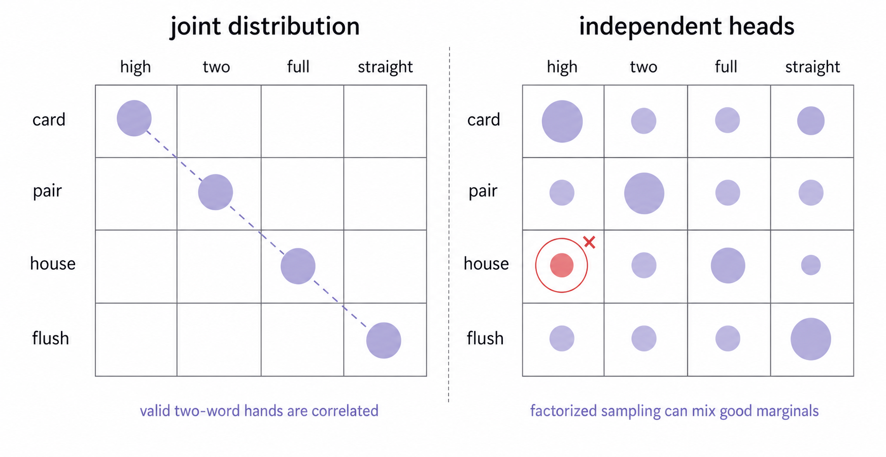
The issue is the independence assumption in the inference process. Current multi-token prediction methods often produce softmax distributions for multiple future positions in parallel, and then sample from those positions independently. This can be useful as part of a larger decoding system, but by itself it does not represent the joint distribution over the tokens being decoded together.

Existing systems often work around this limitation with verification, self-speculative decoding, rejection, or by falling back to ordinary next-token prediction at inference time, as in the DeepSeek-V3 technical report. Those workarounds can be practical, but they also make the capacity issue visible: the inference procedure itself did not directly model the dependency among the tokens.

Continuous-domain language models are especially useful for thinking through the false dichotomy, but they should be separated from masked, discrete, or hybrid diffusion language models. If a language model lives in a continuous state space, then ideas from diffusion and flow matching become available in a more direct way.

Recent examples include Continuous Diffusion for Categorical Data, Flow Map Language Models, CoDAR, LangFlow, ELF, and FlowLM. These methods are not the same object, but they share a broad inference shape: use a continuous state or relaxation before returning to discrete text. They differ in where they place the continuous state, how they map back to tokens, and whether they learn diffusion, flow matching, or a flow-map-like few-step sampler. One remaining challenge is whether these procedures can give a well-defined validation perplexity for text, not only useful samples.

Related reading

• Denoising Diffusion Implicit Models
• Diffusion Forcing
• Block Diffusion
• Diffusion via Autoregressive Models
• Flow Map Matching
• One Step Diffusion via Shortcut Models
• Mean Flows for One-Step Generative Modeling
• Better & Faster Large Language Models via Multi-token Prediction
• Continuous Diffusion for Categorical Data
• Flow Map Language Models
• CoDAR: Continuous Diffusion Language Models are More Powerful Than You Think
• LangFlow
• ELF: Embedded Language Flows
• FlowLM: Few-Step Language Modeling via Diffusion-to-Flow Adaptation
• Sander Dieleman’s “Flow maps”, “Perspectives on diffusion”, and “Diffusion language models”